Bonding Curve Mathematics: From Theory to Pump Fun

Most bonding curves are nothing but CPAMM in disguise

A bonding curve is a mathematical function that defines the relationship between a token’s supply and its price. In Pump.fun’s case, the curve works by increasing the token price exponentially as more tokens are bought using SOL.

There are different types of bonding curves—linear, logarithmic, exponential, and more. Many of these can be derived from or resemble the mechanics of the constant product automated market maker (AMM) formula (like x · y = k). However, not all bonding curves can be expressed through that formula. For example, step-wise pricing curves don't follow a smooth mathematical function, but with slight modifications, similar behavior can be mimicked.

Note: This article should be explored alongside the complete codebase which is heavily inspired from Pump Science Implementaion and the bonding curve visualizer. Together, they provide a comprehensive understanding of the topic.

Now, let’s dive in.

Primer on Constant Product AMM

---

Constant Product Market Maker (CPAMM) works on the following formula:

\(x \cdot y = k \)

Where:

• x and y are the quantities of asset x and asset y, respectively.

• The ratio x / y represents the spot price.

• When a trade occurs, the values of x and y change, but k (the constant product) must remain the same.

Mathematically:

• x = quantity of asset x before the trade

• y = quantity of asset y before the trade

When a user buys token x by sending token y to the pool, the pool adjusts according to this principle:

\((x - x') \cdot (y + y') = k \)

Where:

• x′ = amount of token x sent to the user

• y′ = amount of token y sent by the user into the pool

The value of k remains constant throughout.

Another way to represent this:

Let:

• x = amount of asset a before the trade

• y = amount of asset b before the trade

• x′ = amount of asset a after the trade

• y′ = amount of asset b after the trade

Since both products should equal k, we have:

\(x \cdot y = k \quad \text{(before the trade)} \\ \)

\(x' \cdot y' = k \quad \text{(after the trade)}\)

We can rearrange the formula to solve for x′:

\(x' = \frac{x \cdot y}{y'} \)

This gives us the new quantity of token x left in the pool after the trade.

In an AMM x and y are provided by the liquidity providers but in the case of bonding curve implementation, we introduce an arbitrary amount of x (Virtual Sol Liquidity) and y (Virtual Token Liquidity), allowing us to simulate any liquidity scnerio.

Bonding Curve Code Implementation: Mini Pump

The code implementation for the following explanation can be found in Mini Pump. Follow the code-base alongside this explanation for better understanding.

The main use case for bonding curves today is in launchpads, where tokens can be launched without initial liquidity by selling the minted tokens over an exponential bonding curve — as seen in Pump Fun and Pump Science. Mini Pump is a minimalist implementation of a bonding curve-based launchpad with all the necessary functions:

1. The admin can configure global settings.

2. Anyone can create a token and launch it, minting 1 billion tokens to the bonding curve.

3. Users can buy and sell on the bonding curve.

4. Once 800 million tokens are sold for around desired SOL, the remaining 200 million tokens and all the SOL can be withdrawn by the admin to create a pool on a DEX of their choice. This step can also be automated by making a CPI call directly from the program to the DEX program.

Global config is initialized by the admin post-deployment to define the bonding curve's shape.

• owner → The protocol owner responsible for setting the configuration.

• tokens_to_sell → Total tokens to be sold via the bonding curve (e.g., 800 million).

• total_tokens_to_mint → Total tokens to mint, including tokens for DEX migration (e.g., 1 billion).

• virtual_sol_liquidity (x) → Virtual SOL added to determine the initial price (e.g., 30 SOL).

• virtual_token_liquidity (y) → Virtual tokens used to set the initial price, typically equal to total_tokens_to_mint (e.g., 1 billion).

Each token launch has its own bonding curve account. When a new token is created, the parameters are initialized based on the global config

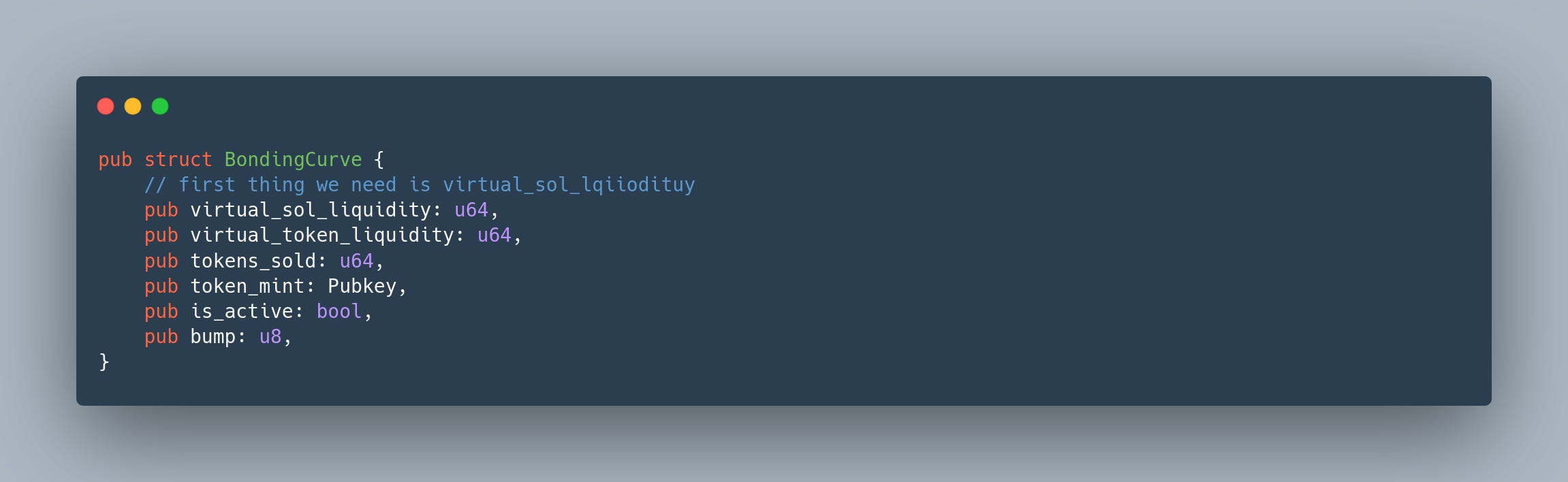
Note the use of virtual liquidity, which distinguishes bonding curve launchpads from traditional AMMs.

Virtual Liquidities serve two main purposes:

• Initial Price Setting
  The ratio virtual_token_liquidity / virtual_sol_liquidity defines the initial price (in tokens per SOL), allowing launches without requiring upfront SOL.

• Curve Shape Control
  These values shape the bonding curve. For example:

  • 300 SOL : 800M tokens results in a linear curve.

  • 30 SOL : 800M tokens results in an exponential curve.

    

You can experiment with different values and see how the curve changes here: Bonding Curve Visualizer

The main point of interest is the functions that calculate the amount of SOL required to buy a certain number of tokens, and the amount of tokens needed to sell into the curve to receive a certain amount of SOL.

You can find the buy and sell logic in the code here: Mini Pump Buy and Sell Calculation Functions

Here is how the formula used in the code is derived:

Let’s say a user wants to buy some tokens for 1 SOL, and the bonding curve for the token has just been deployed.

• virtual_sol_liquidity = 30

• virtual_token_liquidity = 800,000,000

From the AMM formula, we know:

\(x \cdot y = x' \cdot y' \)

\(y' = \frac{x \cdot y}{x + \Delta x} \)

\(y' = \frac{30 \cdot 800{,}000{,}000}{31} = 774{,}193{,}548 \)

\(\Delta y = y - y' = 800{,}000{,}000 - 774{,}193{,}548 = 25{,}806{,}452 \)

Where:

• x: virtual SOL liquidity before the trade

• y: virtual token liquidity before the trade

• x′=x+Δx: virtual SOL liquidity after the trade

• y′: virtual token liquidity after the trade

• Δx: SOL sent by the user

• Δy=y−y′: tokens received by the user

After each trade, we update both virtual_sol_liquidity and virtual_token_liquidity.

Example (Buy Trade)

Initial values:

• virtual_sol_liquidity = 30

• virtual_token_liquidity = 800,000,000

User buys with 1 SOL:

Updated values after trade:

• virtual_sol_liquidity = 30 + 1 = 31

• virtual_token_liquidity = 800,000,000 - ~25,806,452 ≈ 774,193,548

Code reference:
📎 Buy update logic (Line 122)

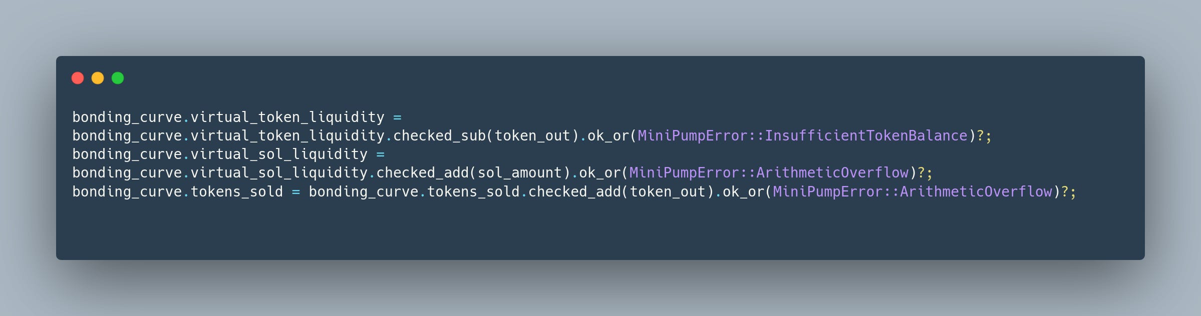
When a user sells tokens to the bonding curve, the logic is exactly reversed.

• Tokens are added back to virtual_token_liquidity

• SOL is subtracted from virtual_sol_liquidity

• Total tokens_sold decreases

Code reference:
📎 Sell update logic (Line 170)

Virtual Liquidity Relationship to Pricing Curve

The greater the token liquidity compared to the SOL, the lower the cost to purchase 800 million tokens — and vice versa.

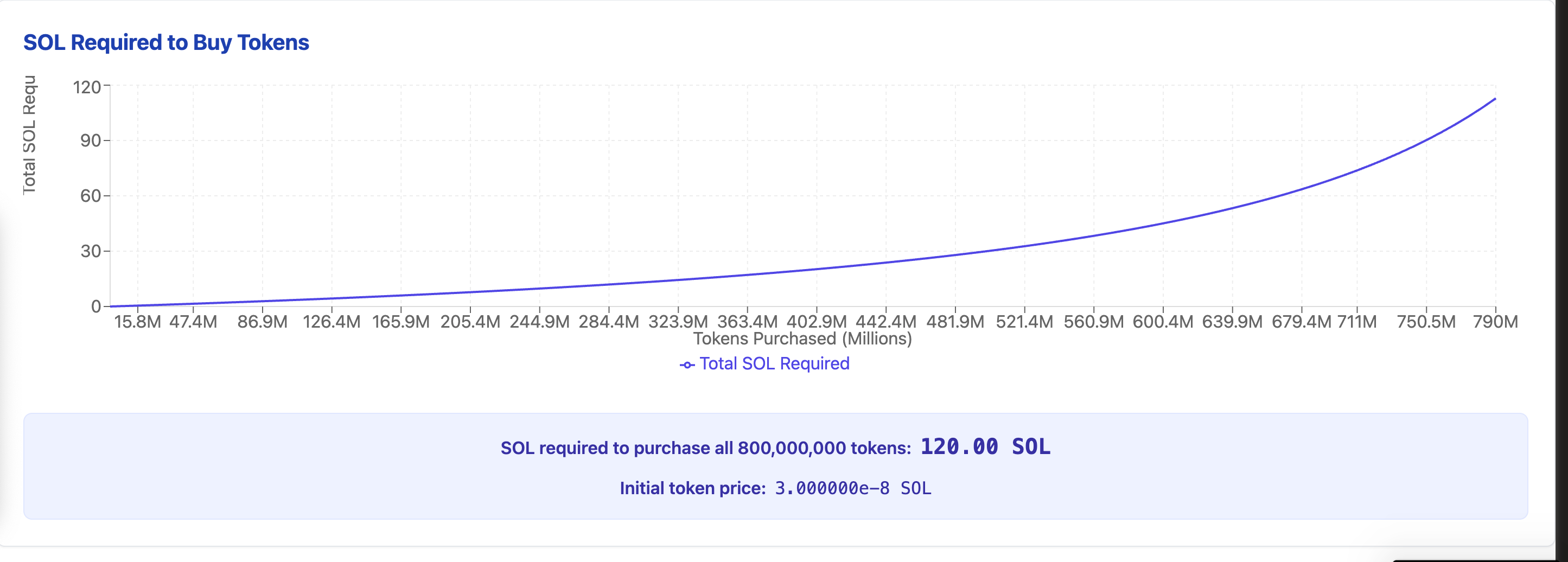
With 1 billion tokens and 30 SOL as initial virtual liquidity, the cost to purchase 800 million tokens would be approximately 120 SOL.

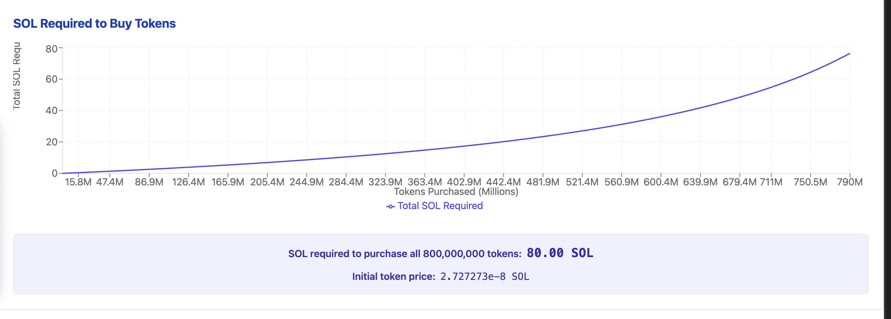
With 1.1 billion tokens and the same 30 SOL in virtual liquidity, the cost to buy 800 million tokens drops to approximately 80 SOL.

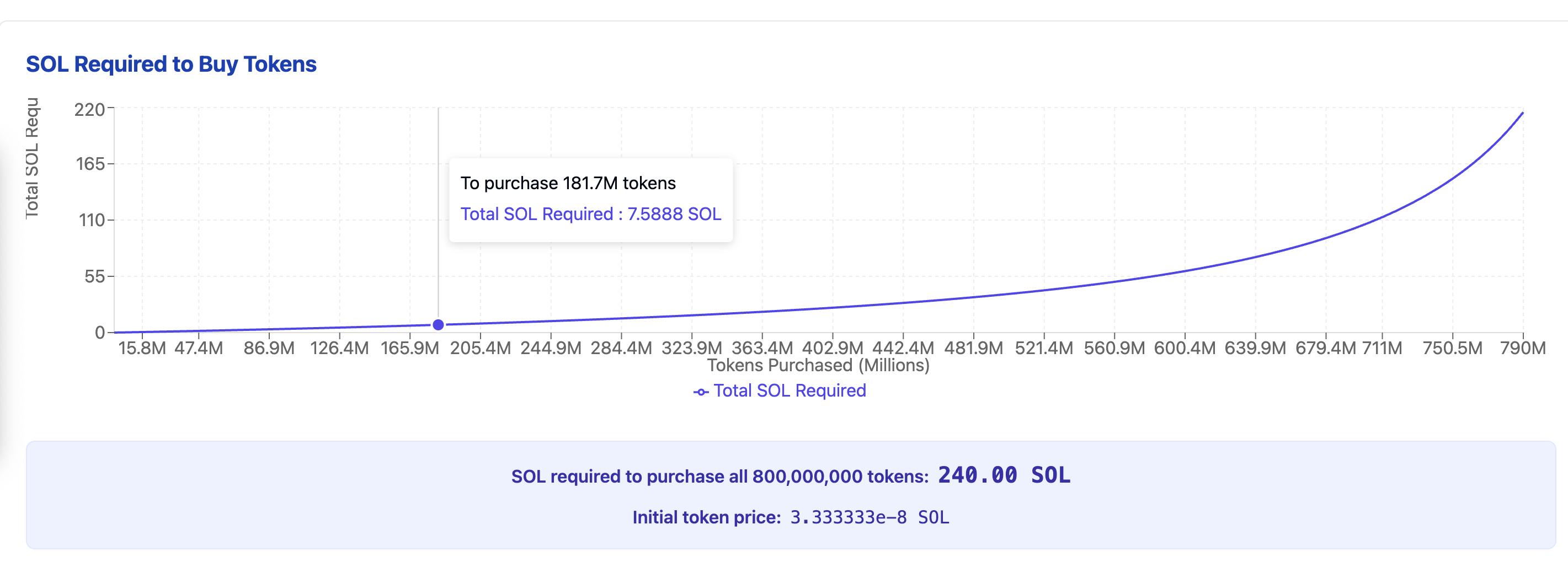
And for 900 million virtual token supply and 30 virtual sol, the price to buy 800 million tokens will be 240 SOL

Edge Case: Setting Entire Virtual Supply Equal to Tokens to Sell

In the case where the virtual token liquidity is set to 800 million tokens, and you try to sell exactly 800 million tokens (effectively reducing the virtual supply to 0), we run into a mathematical issue.

Let's look at the formula:

• x: SOL liquidity = 30 SOL

• y: Token liquidity = 800,000,000 tokens

We know the equation from the AMM formula:

\(x⋅y=x′⋅y′\)

If we attempt to sell 800 million tokens, we have:

\(y′=0\)

Substituting into the formula:

\(x' = \frac{x \cdot y}{y'} \)

\(x' = \frac{x \cdot y}{0} = ∞ \)

Dividing by zero results in an infinite value. Hence, we can never sell exactly 800 million tokens because it would reduce the virtual token liquidity to zero, causing the price to skyrocket to infinity as shown in the chart too.

Problems Bonding Curve Token Launches Solve

Problem 1: Liquidity Barrier to Entry

In an AMM, liquidity for both tokens in the pair is required to enable trading.

For example, Alice creates a token named $ALICE and wants to enable its trading on Raydium by creating the ALICE/SOL pair. The problem is that Alice needs SOL to create the pool. Some might question whether she can just put in a small amount of both tokens in the desired ratio and expect everything to work fine.

In an AMM, the lesser the amount of liquidity, the higher the price impact of trades.

For example, consider a pool with 100,000 ALICE tokens and 1,000 SOL. If a trade of 1,000 ALICE occurs—meaning someone sells 1,000 ALICE tokens in the pool—they will get 9.9 SOL according to CPAMM formula discussed before.

\( x \cdot y = k \)

\(100,000 \cdot 1,000 = 100,000,000\)

\((100,000 - 1,000) \cdot y' = 100,000 \cdot 1,000\)

\(99,000 \cdot y' = 100,000,000\)

\(y' = \frac{100,000,000}{99,000} \approx 1,010.10 \, \text{SOL}\)

\(\text{SOL received} = 1,010.10 - 1,000 = 10.1 \, \text{SOL}\)

But in a pool with 10,000 ALICE tokens and 100 SOL, if a trade for 1,000 ALICE happens—where a seller sells 1,000 ALICE tokens in the pool—they will get only 9.09 SOL.

\(x \cdot y = k\)

\(10,000 \cdot 100 = 1,000,000\)

\((10,000 - 1,000) \cdot y' = 10,000 \cdot 100\)

\(9,000 \cdot y' = 1,000,000\)

\(y' = \frac{1,000,000}{9,000} \approx 111.11 \, \text{SOL}\)

\(\text{SOL received} = 111.11 - 100 = 11.11 \, \text{SOL}\)

Notice that in both cases, the ratio of ALICE to SOL is the same, so the price is similar. However, the user gets a different amount of SOL. The pool with smaller liquidity gives 1 SOL more, which, at the current price of SOL, is around ~$125.

Therefore, the token creator needs a good amount of SOL to create a healthy pool.

Problem 2: Centralized Initial Price Control

Another issue is that, in this case, the creator has full control over the starting price while also holding a large portion of the supply. In contrast, with a bonding curve, the price starts low and gradually increases as a substantial amount of Solana is collected. This is a more inclusive approach, where the community collectively determines whether a token should reach a DEX and start trading at a certain price or die out within the bonding curve.

Security Tips

A common issue I’ve encountered while auditing bonding curve launchpads is that anyone can create the liquidity pool on a DEX, which the launchpad will later migrate to. For example, with Raydium, only one pool is allowed per token pair. If the liquidity migration is automatic through Anchor code, it can result in a denial-of-service (DoS) situation, as the pool is already created.

In this case, instead of attempting to create a new pool (which will fail), you should call the add_liquidity function on the DEX. This function will add liquidity based on the current price that’s already running on the DEX.

---

Feel free to reach out to Nirlin on X for any follow-up questions.